Interactive Geometry and Critical Points
Thomas F. Banchoff [email protected]
Mathematics Department
Brown University
Providence, RI 02912
U.S.A.
Abstract
Interactive geometry programs make it possible to explore critical points of functions of one and many variables, in courses
at various levels and in research projects. In this article, we show how easy-to-use Java applets illustrate
critical point phenomena for families of curves and surfaces from several different viewpoints. Our methods introduce
circular and spherical images of parametric curves and surfaces, leading to results on the tangential degree
of a closed curve in the plane, and the Hopf Theorem on the normal degree of a surface in three-space. We also
indicate the relationship with the basic critical point theorem of Marston Morse concerning pits, peaks, and
passes of a function of two variables.
Introduction
How does an interactive geometry program make it possible to treat a broad subject like critical points of functions
in a unified way, across a wide range of courses at different levels? In this article, we show how coloring the
graph of function of one or more variables can display basic information about the shape of the graph, in particular
the numbers of critical points of different types. A certain amount of information is already available if we
look at a single picture of a function, but we gain a great deal more insight into the geometry of the graph
by interacting with images, in particular by deforming them in a controlled way using special sets of parameters.
In this way we can investigate entire families of functions of one and more variables, showing how the behavior
of critical points changes when we alter the parameters in different ways.
The interactive Java demonstrations presented in this article are intended to illustrate the power of software generated
by teams of students over a period of years under the direction of the author. Running the applets require no
computer algebra system or other commercial software. It is possible for a user to introduce new functions into
the program, although in order to save such modifications it is necessary to be running an expanded program on
a file server. Furthermore it is possible to incorporate programs like those illustrated in this article into
worksheets or laboratory settings for use in conjunction with classes in calculus of one or more variables. We
will not go into detail about the pedagogical implications of using such demonstrations in conjunction with traditional
lecture courses, or in the context of a courseware programs. A report on such efforts, with emphasis on assessment,
is found in the author's paper at the International Conference at KAIST,
Daejon,
Korea
[B2].
At several places in this article we indicate how the same approaches can be used to study more advanced topics in parametric
curves and surfaces, in courses in calculus and in introductory differential geometry and topology.
Readers familiar with the geometry of characteristic classes will recognize ways
in which the examples presented here are fundamental in the study of singularities of mappings of manifolds into
Euclidean spaces, as well as the geometric theory of catastrophes.
1. Graphs of Functions of a Single Variable
We start with the graph of a function of one variable defined over an interval on the real line. By
the simple device of coloring all segments of positive slope red in a polygonal approximation of the function,
and coloring the segments with negative slope white, we can see immediately where the function has local maxima
and minima.Assuming that there are no horizontal segments on the graph, as we move from the left endpoint through
the domain of the function, we can observe when the color of the graph changes, from red to white as we pass
a local maximum and from white back to red at a local minimum. If we start with a red segment and end with a
white one, then there must be an odd number of color changes, so there are an odd number of critical points in
the domain. The number of local maxima is one greater than the number of local minima and in particular there
is at least one local maximum. Similarly, if the segments at the endpoints of the interval have the same color,
then the number of critical points in the interval is even, with the same number of local maxima as local minima.
So far these observations depend on studying the changes of slope from positive to negative or conversely in
a polygonal approximation of a function, and this can be done in a course in pre-calculus mathematics.
In a course in calculus of one variable, the corresponding results are expressed in classical theorems. For the graph of
a differentiable function of one variable f(x), the number of points c where f'(c) = 0 in the interval [a,b]
is even if f'(a) and f'(b) have the same sign and this number is odd if the signs are different, (assuming that
there are a finite number of critical points in the interval and that the sign of the derivative changes as we
go from left to right past a zero of the first derivative). Beginning students will appreciate the difference
in two basic examples: the function f(x) = x2 has an odd number of critical points in
the interval [-2,2] since f'(x) = 2x so f'(-2) and f'(2) have different signs; on the other hand, the function
f(x) = x3
- 3x has f'(x) = 3x2
- 3 so f'(-2) and f'(2) are
both positive and the function must have an even number of critical
points in
the domain, in this case two.
For the graph of a differentiable function, we can describe the coloring scheme in a different way that will be useful in
our generalizations. The normal line at a point of the graph of a differentiable function is perpendicular to
the tangent line to the function graph at the point. For each point,
the unit vector pointing upward from the origin that is parallel to the normal line at the point is called the
"circular image" of the point. If we color the left half of this upper semicircle red and the right half white,
we can reinterpret the coloring introduced in the previous paragraph by saying that a point on the graph is given
the same color as its circular image.
It is easy to illustrate the color scheme described above by showing a few pictures. What can interactive computer graphics
add to the experience of the teacher and the students? With interactive
graphics, we can carry out online investigations of families of functions depending on one or more parameters.
We present some simple examples of this procedure, and then show how to use the same setup for more advanced
investigations. We will confine ourselves to polynomial functions in the introductory parts of the paper, and
introduce trigonometric examples when we study parametric curves and surfaces.
As examples of such families, we can see what happens as we change the coefficients of polynomials. For
linear functions, f(x) = mx + b, changing the slope m will just rotate the line about its y-intercept, and changing
the y-intercept b will move the graph up and down without altering its shape. Also making a change in the domain
gives us a function g(x) = f(x+h) = m(x+h) + b = mx + (mh+b), which moves the graph right or left, keeping the
slope the same. If m is not equal to zero, we can choose h = -b/m so the equation takes the simple form g(x)
= mx.
For a quadratic function f(x) = ax2 + mx + b with a positive, the graph is a
parabola
opening upwards and with a negative, a parabola opening downwards. Changing the constant term
b shifts the graph vertically. A change from x to x+h shifts the graph horizontally without changing its shape,
and g(x) = f(x+h) = a(x+h)
2 + m(x+h) + b = ax
2
+ (2ah + m)x + (ah2 + mh + b). If a is
non-zero, we can choose h = -m/2a so
that the equation takes the form g(x) = ax2
+ (-m2/4a + b), with no
linear
term and with the graph symmetric with respect to the y-axis.
2. The Family of Cubic Equations
What about cubic equations of the form f(x) = x3
+ ax2 + mx + b? As
before, in order to shift right or
left,
we set g(x) = f(x+h) = (x+h)3 + a(x+h)
2 + m(x+h) + b = x3
+ (3h + a)x
2 +
3h2 + 2ah + m)x + (h3
+ ah2 + mh + b).
By choosing h = -a/3 we obtain a function of the form g(x) = x3
+ Mx + B, where M and B are constants that we can manipulate. If we choose B = 0, we have a one-parameter family of cubics
with no squared term and no constant terms. Any cubic
will have the shape of exactly one of the cubics of this special form.
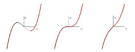
Students can now investigate functions of the form f(x) = x3
+ mx by changing the parameter m and observing the numbers of critical points of the graph. Immediately
we are led to the conjecture that when m is positive, there are no critical points for the function and when
m is negative, the number of critical points is two. Students can prove this conjecture can then be proven by
finding the derivative f'(x) = 3x2 + m, which will never be zero if m is positive
and which
is zero for exactly two values of x when m is negative.
The intermediate case, with m = 0, has a
horizontal inflection point at the origin when x = 0.
The value x is called a "degenerate"
critical point, since f'(0) = 0
so the tangent line is horizontal, but f'(x) is positive for all other
x, so
the sign of the derivative does not change at the critical point, the
way it
does for a local maximum or minimum.
The color coding introduced in the previous paragraphs makes it easy to see how the critical point behavior changes as we
change the value of m in an interactive demonstration. The Java applet
following the first illustration makes it possible for a teacher and students to investigate this behavior by
changing the "slider bar" that gives the value for m.
In addition to indicating the slope of the tangent line, we can color the points on the graph by a darker color when the
slope of the tangent line is negative, so we have a visual record of the places where the slope changes from
positive to negative (the local maxima of the curve, colored with a darker
color) and where it changes from negative to positive (at the local minima, with lighter color).
Note that f''(x) = 6x no matter what m is, so the concavity of the graph changes from convex downward to convex upward as
x goes from negative values to positive values in the domain.
By making
the graph thick when the second derivative is positive and thin where it is negative, we can observe the inflections
points of the graph, where the second derivative changes sign and the concavity of the graph changes.
Figure 1: The family of cubic equations
3. The
Family of Quartic Equations
More interesting is the case of a quartic, or fourth degree polynomial f(x) = -x4 + cx3 + ax2 + mx + b. As in the case of the quadratic and the cubic, changing b only shifts the y-intercept
up and down without changing the shape of the curve. Also, shifting the domain by setting g(x) = f(x+h) = -(x+h)4 +c(x+h)3 + a(x+h)2 + m(x+h) + b = -x4 + (6h +c)x3 + lower order terms,
so choosing h = -c/6 we can eliminate the coefficient of x3. As usual we can shift vertically by choosing
the constant to be zero, so the graph of any quartic function of this type can be written, f(x) = -x4 + ux2 + vx, for appropriate choices of the parameters u and v.
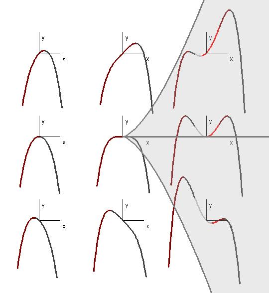
Once again, an interactive graphics programs makes it possible for students to explore the family of graphs of quartic functions
by choosing values u and v in the "two-dimensional control space". Sometimes the number of critical points is
1, for example when v = 0 and u is negative, and other times there are 3 critical points, for example when v
= 0 and u is positive. What happens if v is not zero? When will we get 3 critical points and when will we get
1? Will we ever get exactly 2 critical points?
If v = 0, then we observe that for any positive number u, the graph will have three critical points, two minima and one local
maxima. We can show this algebraically by computing f'(x) = -4x3 + 2ux = -2x(2x2 -u), which will equal zero for at x = 0 and at two other values of x if u is positive, and only at x = 0 if u
is positive.
If we choose u = 1 so that f(x) = -x4 + x2 + vx, then for some values of v near zero, the
number of critical points is still 3, but for some values of v, the number of critical points changes to 1. We
can observe that this change occurs at the value of v for which the function has a horizontal inflection point,
where f'(x) = 0 and f''(x) = 0. Thus we must have both f'(x) = -4x
3 + 2x + v = 0 and f''(x) = -12x2 + 2 = 0. From the second equation, x is plus or minus
the square root of 1/6, so v = ±(4/3)√(1/6). For general u, we obtain the equations f'(x) = -4x3 + 2ux + v = 0 and f''(x) = -12x2 + 2u = 0 so |x| = √u/6 and v = 4x3 style="color:
black;"> - 2ux = (4u/6)√u/6 - 2u√u/6 = -(4/3)u√u/6. Therefore 27v2 = 8u3.
This "semi-cubical parabola" curve in the "control space" of all possible choices of u and v will separate the
(u,v) choices that give functions with 3 critical points from those that give functions with 1 critical point.
We can use the interactive graphics system to construct a collection of function graphs that exhibit the different configurations
of critical points for different choices of u and v.
Figure 2: The family of quartic equations
Mathematicians familiar with catastrophe theory will recognize that these two families of functions, the cubic curves and
the quartic curves, are two of the most important basic examples in that theory.
Originally
arising in the sciences of optics and structural design, catastrophe theory has significant applications in physics
and engineering and in differential geometry and other parts of mathematics.
It is noteworthy that interactive computer graphics makes it possible to introduce this modern subject to students
just beginning the study of calculus and analytic geometry for functions of one variable.
For a good introduction to elementary catastrophe theory for functions of one variable,
see
the Catastrophe Teacher website of Lucien Dujardin
http://pagesperso-orange.fr/l.d.v.dujardin/ct/eng_index.html.
4. Critical Points for Parametric Curves
There are two natural ways to extend the analysis of functions of a single variable to more general situations: either we
may consider parametric curves in the plane, or we can consider graphs of functions of two variables in three-dimensional
space, eventually moving on to study parametric surfaces.
For a differentiable closed curve in the plane given in parametric form by (x(t),y(t)) with t going from a to b, there is
a velocity vector (x'(t),y'(t)) at each point, and a normal vector (-y'(t), x'(t)) perpendicular to the velocity
vector.
The unit vector in the direction of the normal vector is called the "circular image" at the point.
In contradistinction to the case of a function graph where all the circular images were
in the upper semicircle, in the case of a parametric curve, any point on the unit circle can be the circular
image of a of a point on the curve.
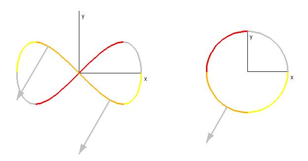
If, as before, we color red the points of the unit circle to the left of the vertical and if we color
the points in the lower semicircle yellow, then the first quadrant will be white, the second will be red, the
third will be orange, and the fourth will be yellow. We can then color each point
on the parametric curve with the same color as its circular image.
We can then read off the critical points of the horizontal coordinate function x(t) by finding points where the color changes
from yellow to white or from red to orange, or conversely.
The critical
points of other coordinate function y(t) on the other hand occur where the color changes from white to red or
from orange to yellow or conversely.
The number of color changes for each of the
two coordinate functions will be even and the total number will be even.
This is
true whether or not the curve intersects itself.
Figure 3: Color-labeled parametric curves in the plane
As the point (x(t),y(t)) moves along the curve, the corresponding unit normal vector on the unit circle is either moving
counterclockwise or clockwise, and we can indicate this by making the curve thin in the first case and thick
in the second case. The points of the curve where the direction changes
are the inflection points of the curve. Students can investigate various curves,
and observe the number of points on the curve that correspond to any chosen point on the circle. How
does the number of corresponding points change as we move the position on the circle? What
happens as we pass a point on the circle that corresponds to an inflection point on the curve?
The investigation of curves in the plane leads to the theory of tangential degree of a curve, an important concept
in the differential geometry of curves in the plane.
5. Families of Parametric Curves
Just as we considered one- and two-parameter families of function graphs, we can explore families of closed parametric plane
curves like the cardioid family: (-(u+cos(t))cos(t),(u+cos(t))sin(t)).
Students can discover that the shapes of these curves depend on u and in particular, that the shape changes
dramatically near u = 1 and -1.
As we watch an animation of this family as u runs
from u = .6 to u = 1.4, we can observe that the curve has a loop for u less than 1, then a cusp at u = 1 and
then a pair of inflection points and finally a convex curve. Students can also record what happens near other
significant points, when u = -2, -1, 0, 1, and 2. For u between -1 and 1, the circular image of the parametric
curve covers the unit circle exactly twice, while for u greater than 1 or less than -1, the unit circles is covered
once algebraically. For u between 1 and 2, or between -1 and -2, there are inflection points where the circular
image doubles back on itself, so that some points of the circle are the circular image of three points, two where
the image curve travels in a counterclockwise (positive) direction and one where it travels in a clockwise (positive)
direction, whereas all but two other points on the circle are the circular image of exactly one point on the
curve, where the image curve travels in a positive directions. We say that such a curve has "tangential degree
1", a concept of great importance the in differential geometry and topology of plane curves
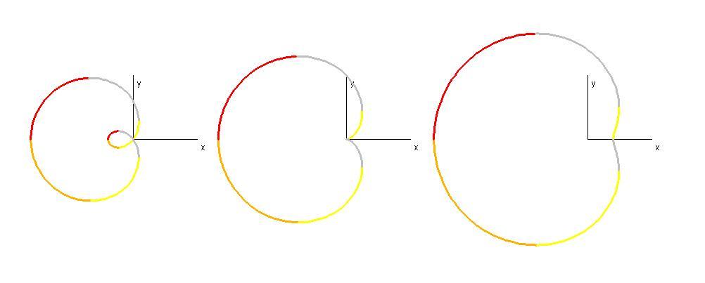
Figure 4: The cardioid family, color-coded
6. Critical Points and Functions of Two Variables
We can generalize the study graphs of functions of one variable in the plane to the study of graphs of functions of two variables
in three-space. We restrict ourselves to functions defined on simple
domains such as a rectangle or circular disc. As in the case of functions of one
variable, we want to find the range of a function, namely the smallest rectangular or cylindrical prism (called
a "box") over the domain that will contain all of the function values for points in the domain. A
point of the graph in the top plane of such a box will correspond to either an interior point of
the domain or a point on the boundary curve.
If the function is differentiable, then a point of the graph in the top plane corresponding
to an interior point will have the top plane as its horizontal tangent plane, and for an interior global minimum,
the bottom plane of the box will contain the horizontal tangent plane at the point of the graph.
On the other hand, it might be that the highest or lowest point occurs at a point on the boundary curve of the domain,
and in that case the tangent line to the boundary curve will be a horizontal tangent line lying on the top or
bottom face of the containing box.
In addition to the local maxima of functions of two variables, represented by the origin in the function f(x,y) = -x
2 - y2
and the minima represented by the origin for f(x,y) = x2
+ y2,
there are other points where the tangent plane is horizontal, for
example the
origin in the saddle-shaped graph of f(x,y) = x2
- y2, defined either over a
square domain or a circular disc domain centered at the origin. This is a typical "ordinary saddle
point" for the graph of the function. Finding the critical points of a function includes finding all local maxima,
local minima, and saddle points.
There are other types of critical points such as the origin for f(x,y) = x
2
- y3 or f(x,y) = x3
- 3xy
2, but these are "degenerate" and can be
eliminated by deforming the
function in a way we will make precise in our examples.
An important theorem of Marston Morse states that, for almost all functions of two real variables, the only critical
points that occur are local maxima, local minima, or ordinary saddle points.
Two particular examples of polynomial functions give a good idea of the critical point behavior for functions of two variables.
Both are named for geographical features: Twin Peaks and
Crater Lake. These surfaces are described in the author's Scientific American Library volume "Beyond
the Third Dimension" [B].
7. Twin
Peaks the Geometry of Peaks and Passes
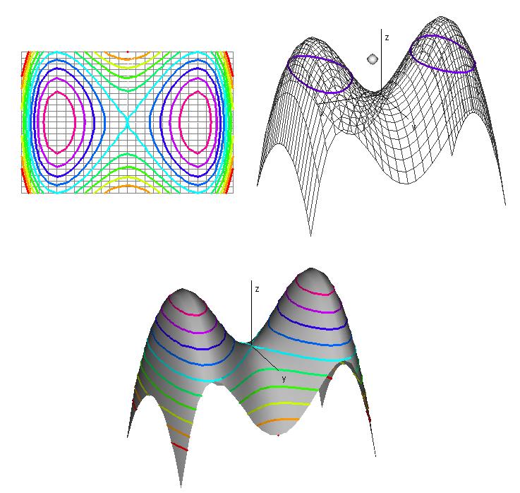
Twin Peaks
is the graph of the function f(x,y) = -x
4
+ 2x2 - y2
over the domain -1.5 ≤ x ≤ 1.5, -1 < y < 1. Even
without any calculus, it is straightforward to show algebraically that f(x,y) ≤ 1 and that equality occurs
at two "peaks" (1,0) and (-1,0). Between the two peaks there is a saddle point at
(0,0), and there are no other critical points for the function. The level set for
z = 1 consists of the two points (1,0) and (-1,0). For 0 < z < 1, the level
set consists of two closed curves.
The level set for z = 0 is a self-intersecting "figure eight" curve, and for z < 0, the level set the portion of
a single closed curve inside the rectangular domain. These level set phenomena can
be investigated with a Java applet:
Figure 5: Graph and slices of Twin Peaks
This kind of "level set analysis" is central to an interactive graphics approach to graphs of functions of one or more variables.
Students can investigate function graphs and report their observations on worksheets or
by online messages.
They can make conjectures about various configurations that arise in graphs of certain kinds of equations,
and then go on to find algebraic reasons for these observed phenomena.
For
Twin Peaks, we can observe that the two local maxima are at the same height, a situation that can
be removed by a slight perturbation.
In geographic terms, we may consider the effect of a slight "earthquake", a shearing transformation obtained by adding
a linear term mx to the equation for f(x,y) = -x4 + 2x
2 - y2
. In the study of functions of one variable, we can add
a linear term to the function f(x) = -x + 2x2 to get f(x) = -x
4
+ 2x2 + mx, and a small non-zero m gives a
function with two local maxima at different heights. The same thing
happens for
Twin Peaks. For small m, the graph of
f(x,y)
= -x4 + 2x
2 + mx - y2
has two peaks at different heights. When the parameter
m is large enough, for an "extreme earthquake", the number of peaks goes from two to one and the saddle point
disappears. Just as in the case of one variable, students can identify by observation where that crucial changeover
occurs then find the values of m for which the function has a degenerate critical point, the analogue of a horizontal
inflection point.
8. Crater Lake and the Geometry of Pits and Passes
Crater Lake
exhibits a different kind of unstable situation.
The graph of g(x,y) = -(x
2
+ y2)
2
+ 2(x2 +
y2) is a surface of revolution about the z-axis
with profile curve -x4 +
2x2. The maximum
value of this function is 1, and there are infinitely many global maxima, lying over the circle x
2 +
y2 = 1 in the domain. There
is one local minimum at the origin. Once again an earthquake shear will perturb this
situation to give the graph of g(x,y) = -(x2
+ y2)
2 + 2(x2
+ y2) + mx, which will still have one local minimum,
but the
circle of maxima will break up into one global maximum and one saddle
point, at
least if m is small enough. The level set at the local minimum will be an isolated point surrounded
by a single level curve.
The level set at the global maximum will be a single point, and the level set at
the saddle point will be a "double loop with a single crossing point".
Near the saddle point, the level set looks like a pair of intersecting lines, as
in the case of the figure-eight curve for
Twin Peaks. Between the level of the maximum and the saddle, the level set is a single curve. Between
the saddle and the local minimum, the level set consists of two curves, one inside the other (as opposed to next
to each other as in the case of
Twin Peaks
). Below the local minimum, the level set is again the part of a single
curve lying in the domain.
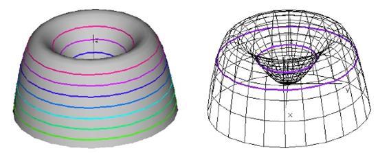
Figure 6: Graph and slices of Crater Lake
This description of the critical points configuration assumes that the earthquake has not been too severe.
If the number m becomes large enough then we obtain a function graph with one global
maximum and no other critical points.
The local minimum and the saddle point have come together and disappeared.
The water in
Crater Lake has spilled out. Students can find this point by observation (and compare the value of
m with m that produces a surface with a degenerate critical point in the case of
Twin Peaks).
9. The Critical Point Theorem for Graphs of Functions of Two Variables
Both of these topographical examples suggest ways of designing function graphs with other configurations of critical points,
say with n+1 local maxima and n saddle points in between.
Then we can introduce m local minima and m ordinary saddles, of the type found
in the tilted
Crater Lake
. This will produce a function graph with n+1 maxima, n + m saddles and
m minima, so in particular the number of maxima plus the number of minima is one greater than the number of saddles,
and the total number of critical points will be an odd number.
We can collect these observations in a conjecture: For an "island" defined over a
region in the plane with one boundary curve at sea level zero and all other points on the island above sea level,
there will be at least one global maximum.
Furthermore, if all critical points are local maxima, local minima, and ordinary saddles, then the number of critical
points is odd and moreover #maxima - #saddles + #minima = 1. This conjecture epitomizes
fundamental results in Critical Point Theory, of immense importance in global geometry and analysis over the
last 80 years. It is also of fundamental importance for the geometry of surfaces,
leading to a modern proof of the crucial Gauss-Bonnet Theorem as well as properties of knotted "strings" in contemporary
molecular biology and theoretical physics.
The mathematician who popularized critical point theory was Marston Morse in a series of articles on the subject
eighty years ago. He enjoyed giving popular lectures on the topic for students of
all levels, and two of his previously unpublished presentations appeared in the November 2007 issue of The American
Mathematical Monthly [M]. On a visit to
Providence
RI
in the 1970's, he came to the computer graphics laboratory at
Brown
University
where my computer scientist colleague Charles Strauss and I were developing a program for analyzing the geometry of surfaces
in three and four dimensions.
Although the graphics programs were primitive by today's standards, and very slow,
Marston Morse immediately appreciated the potential of such approaches for teaching, research, and public exposition
of geometric ideas arising in critical point theory.
We could not carry out those projects forty years ago, but now they are possible
using interactive geometry programs and Java applets.
10. Color-Coding Graphs of Functions and Partial Derivatives
When we analyzed level sets of functions of two variables, we used a spectrum of colors to indicate the heights of the slices.
For the subject of partial derivatives, we need only two colors for each variable,
four in all.
Just as we colored graphs of functions f(x) in the plane by red or white depending
on the algebraic sign of f'(x) or the position of the unit normal vector in the left or right side of the circular
image, we can color the graph of a function f(x,y) depending on the signs of the partial derivative functions
f
x(x,y) and fy(x,y). For
a differentiable function there is a well-defined tangent plane at each point of the graph and an upward-pointing
normal perpendicular to that plane.
If fx(x,y)
and fy(x,y) denote the first
partial derivatives of f with respect to x and y respectively, then
(-fx(x,y),-fy
(x,y),1) will be a normal vector.
We can color the surface white if fx(x,y)
is positive and red if it is negative
in order to exhibit the points separating those regions, where fx
(x,y) = 0.
Geometrically speaking, a point has f
x(x,y) = 0 if its tangent plane is perpendicular
to the y-z-coordinate
plane. Similarly if we color the surface white if fy
(x,y) is positive and blue if it is negative, we can identify the points where f
y
(x,y) = 0, and where the tangent plane is perpendicular to the x-z-plane.
We can then use additively to color the surface purple where it is both red and blue, where fx
(x,y) and fy(x,y) are both positive.
The surface will be colored red when fx(x,y)
is positive and fy(x,y) is
negative, and blue when when fx(x,y) is negative and f
y(x,y)
is positive. If both fx(x,y)
and fy(x,y) are negative, the
surface is colored white. Thus we color a point white, red, purple, or blue as the point (-f
x(x,y),-fy
(x,y)) lies in the first, second, third, or fourth quadrant in the plane.
A point will be a critical point if all four colors meet at the point.
We can also
express this condition by saying that the point is in the intersection of the locus f
x
(x,y) = 0 and the locus fy
(x,y) = 0. Usually those conditions are expressed and dealt with only algebraically, but interactive computer
graphics provides a direct visual display of the geometric properties of these partial derivative functions.
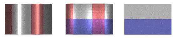
Figure 7:
Perturbed Twin Peaks, color-coded domains
We obtain a bonus from this method of coloring because we can tell whether a critical point represents a maximum or minimum
on one hand or a saddle point on the other.
In the first case, the four regions at a point are red, purple, blue and white in counterclockwise order, while in
the second case, the cyclic order is red, white, blue, and purple. The difference
between these two orderings is connected with the sign of the spherical image mapping defined on the surface,
originally introduced by Gauss.
This method of visualizing critical point configurations is especially helpful when we are exploring one-parameter families
of functions, for example the perturbations of Twin Peaks.
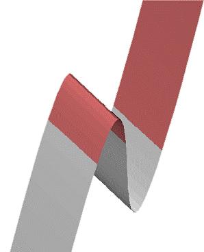
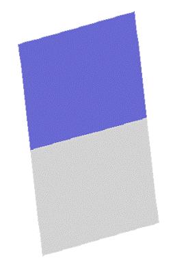
Figure 8:
Color-coded partial derivative graphs for Twin Peaks
The picture on the left shows the graph of the first partial derivative of f(x,y) with respect to x, colored to indicate
where the value of that function is positive.
The colored region is separated from the uncolored region by curves indicating where the f
x
(x,y) = 0. The picture on the right shows the corresponding
graph for the first partial derivative with respect to y.
The colored region indicates where fy(x,y)
is
positive, and that region is bounded by the curve where fy(x,y)
= 0.
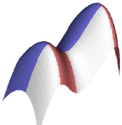
Figure 9:
Color-coded graph of perturbed Twin Peaks
The graph of the perturbed Twin Peaks function colored according to the signs of the two first partial derivatives has four
different colors near any critical point of the function, where the curves corresponding to f
x(x,y) = 0 and fy
(x,y) = 0 intersect.
11. Perturbations of the Graph of Crater Lake
We can carry out the same analysis for the
Crater Lake function to show the graphs of the two first partial derivatives.
In the domain, we have a pair of curves where fx(x,y)
= 0 and a pair of
intersecting curves where fy(x,y) = 0.
The intersections of these two pairs of curves yield three critical points, one global maximum, one ordinary saddle,
and one local minimum.
Note the in the unperturbed
Crater Lake, all of the points on the top rim of the graph represent global maxima.
The
curve of points where both partial derivatives are zero will be purple on one side and white on the other, or
red on one side and blue on the other.
This is a degenerate situation since the curves
where f
x(x,y) =
0 and fy(x,y) = 0 coincide. When
we introduce a shear by adding mx for small x, these two loci are perturbed so that they intersect at a finite
number of points, with all four colors in a neighborhood of each of these critical points.
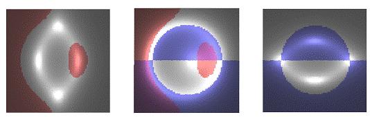
Figure 10:
Perturbed Crater Lake, color-coded domain
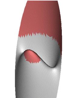
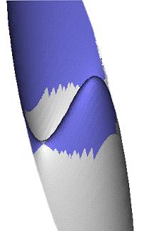
Figure 11:
Color-coded partial derivative graphs for Crater Lake
Figure 12:
Color-coded graph of perturbed Crater Lake
The graph of perturbed Crater Lakes function colored according to the signs of the two first partial derivatives has four
different colors near any critical point of the function, where the curves corresponding to fx(x,y)
= 0 and f
y(x,y) = 0 intersect.
12. Parametric Surfaces in Three-Dimensional Space
Just as we can generalize from graphs of functions of one variable to closed parametric curves in the plane, we can generalize
from graphs of functions of two variables to parametric surfaces in space. For
such surfaces, the outer normal vector can point into the upper hemisphere where the coloring is white, red,
purple, and blue, or into the lower hemisphere, for which directions the color is yellow, overlaid as appropriate
with red to make orange, or blue to make green, or purple to make brown.
The eight quadrants of the unit sphere are then color-coded in such a way that a small polygonal region on a surface
receives the color of the octant within which its outward normal vector lies.
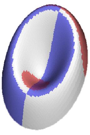
Figure 13: A torus held vertically
Note that for the torus of revolution, the critical points of vertical coordinate function have a local maximum at an entire
circle, similar to the situation at the top rim of the Crater Lake functions graph. We can obtain isolated
critical points either by rotating the torus or by perturbing it by adding a multiple of sin(2u) to get two global
maxima or a multiple of sin(3u) to get three local maxima. Once again the critical points of the coordinate
functions will occur when four different colors come together on the surface, when the color of the surface corresponds
to the color of the normal vector to the surface on the unit sphere.
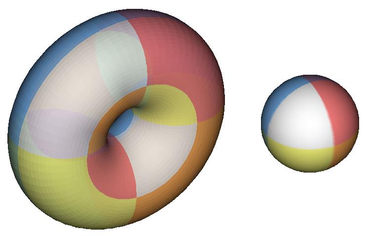
Figure 14: Warped torus - torus plus multiple of sin(2u)
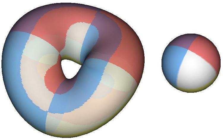
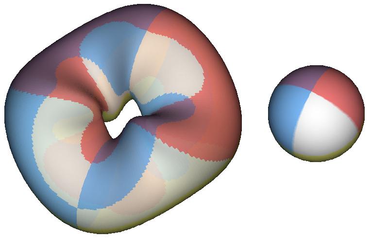
Figure 15: Warped torus - torus plus multiple of sin(3u)
When a neighborhood of a point is colored with red, white, blue and purple, or the same four colors in the opposite
order, the spherical image of the point is the north pole, the unit vector along the positive z-axis. When the
coloration is orange, yellow, green, and brown, or these colors in the opposite order, the spherical image of
the point is the south pole. The Hopf degree theorem states that the algebraic number of times that the north
pole is hit is the same as the number of times that the south pole it hit, where the first ordering is counted
positively and the second negatively. Each of these numbers is half of the "Euler characteristic of the surface",
a number that expressed the complexity of the shape of the surface. This result is basic in the topology and
geometry of surfaces, and it is fundamental to the modern theory of extrinsic differential geometry of surfaces.
Just as Morse would be pleased to see interactive demonstrations of critical points, Gauss would appreciate interactive
exploration of surfaces in three-space and higher. Such topics will be dealt with in later papers on interactive
geometry in differential geometry and combinatorial topology.
Conclusion
Interactive computer graphics makes it possible to investigate phenomena connected with critical points of functions in the
plane and in three-dimensional space, starting with elementary calculus and proceeding to theorems in differential
geometry and topology. These techniques have great potential for engaging students and general audiences as well
as providing fruitful areas for research, in pedagogy as well as geometry and topology.
Acknowledgements
Special thanks are due to Michael Schwarz, who wrote the Java demonstrations used for the illustrations in this article, and to Frederick Choi, who updated them.
The software for the Java applets was created at
Brown
University
by David Eigen under the direction of the author.
References
|
[B1] |
|
Banchoff, Thomas "Beyond the Third Dimension"
(1990) Scientific American Library, Freeman Publishing Co.
|
|
[B2] |
|
Banchoff, Thomas, "Interactive Geometry and
Multivariable Calculus on the Internet" CBMS Issues in Mathematical
Education, Vol. 14 (2007), p. 17-31.
|
|
[M] |
|
Morse, Marston, "Topology and Equilibria"
(November 2007) The American Mathematical Monthly, p. 819-834.
|